—Ann E Nicholson
Since Bayesians without Borders will in significant part be about Bayesian networks and their uses, in this post I will introduce them to newcomers to the technology.
Bayesian networks (BNs) are an increasingly popular technology for representing and reasoning about problems in which probability plays a role. A Bayesian network is a directed, acyclic graph whose nodes represent random variables and arcs represent direct dependencies. The arcs often, but not always, also represent direct causal connections between the variables. The nodes pointing to  are called its parents and collectively are denoted
  . The relationship between variables is quantified by conditional probability tables (CPTs) associated with each node, namely
  . The CPTs together compactly represent the full joint distribution. Users can set the values of any combination of nodes in the network that they have observed. This evidence,
  , propagates through the network, producing a new posterior probability distribution
  for each variable in the network. There are a number of efficient exact and approximate inference algorithms for performing this probabilistic updating, providing a powerful combination of predictive, diagnostic and explanatory reasoning.
I will illustrate with the design of a BN for a simplified version of a real ecological problem, modeling native fish populations in Victoria. Problem: A local river with tree-lined banks is known to contain native fishpopulations, which need to be conserved. The river passes through croplands and is susceptible to drought conditions. Rainfall helps native fish populations by maintaining water flow, which increases habitat suitability as well as connectivity between different habitat areas. However, rain can also wash pesticides that are dangerous to fish from the croplands into the river. What we want to do is build a BN adequate for modeling this system.
The first step is to decide what the variables of interest are, which will become the nodes in the BN. The abundance of native fish directly depends only on the level of pesticide in the river and the river flow, hence Native Fish Abundance — a so-called "leaf node" — has only those two parent nodes. RiverFlow depends on how much rain falls in a given year (Annual Rainfall), and how much of that water ends up in the river, which means it depends also on the long term Drought Conditions. The amount of pesticide in the river (Pesticide in River) depends on Pesticide Use and whether there is enough rain (Annual Rainfall) to wash it into the river. Finally, the condition of the trees on the river bank depends only on the long term drought and more recent rainfall.
This graphical structure captures these causal interactions: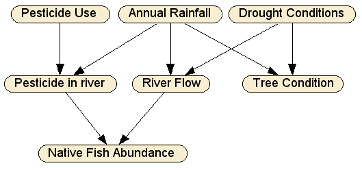
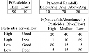
In consultation with an ecologist we might build the CPTs (i.e., eliciting the parameters from the ecologist), as in these example tables:
Note that Pesticide Use (just "Pesticides" in the table) and Annual Rainfall are so-called "root nodes" with no parents, so there is only a single probability distribution for each, whereas for nodes with parents there is a conditional distribution for each possible instantiation of its parents.
The CPT for the Native Fish Abundance node shows the possible combinations of values for the parent nodes (Pesticides and River Flow), and a probability distribution of the resultant Native Fish Abundance, over the three levels, High, Medium and Low. We can see that the best conditions for the fish are Low levels of pesticide and Good River Flow (.8, .15, 0.05), while the worst are High pesticide use and Poor River Flow (.01, .10, .89). Note also that there may well be other factors in play, such as the presence of exotic predators, or disease, that are not represented explicitly by nodes in the BN. The effects of these are averaged over in the CPTs. They are reflected, for example in the 0.05 probability that native fish abundance is Low, even under the best pesticide and river flow conditions.
Now that we have the BN structure and its parameters, the BN can be used for reasoning. That is, we can instantiate different possible scenarios by updating the values of particular nodes and then updating the BN, using one of the many Bayesian network programs around, such as Netica. First, here is the network with no evidence:
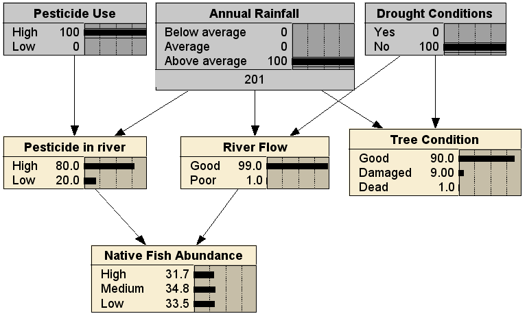
Without making any observations, this BN tells us that the most likely state of the native fish is Low abundance (57.8%), though the Tree Condition is most likely Good (53.3%). If we add observations of the root nodes in the BN, when there is High pesticide use, above average rainfall and no drought conditions, we get:
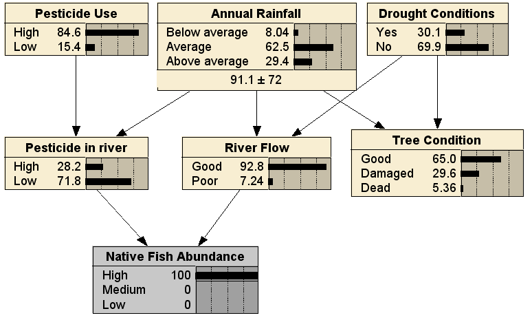
This reasoning is predictive, from cause to effect. In this scenario, the prediction is that the Native Fish Abundance will improve, due to the River Flow being Good, despite the increased Pesticide in River. Alternatively, the BN can be used for diagnosis, by entering evidence for the Native Fish Abundance leaf node:
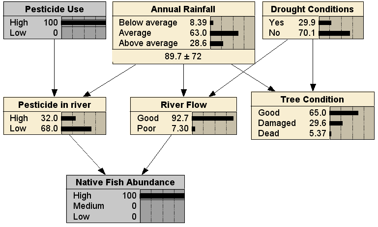
Comparing to the no evidence case, we can see that it is less likely that the pesticide use was high, less likely there have been drought conditions, and more likely that rainfall has been above average. Finally, we can use the BN in any arbitrary combination of diagnostic and predictive reasoning; here with evidence entered for both a cause (Pesticide Use being High) and an effect (Native Fish Abundance being High), resulting in (fairly small) changes to the distributions for all the other nodes:
Here I have briefly described and illustrated the usual knowledge engineering process of building Bayesian networks. There is, of course, a great deal more to it when building a real network of any complexity, which you can read about in depth in our book Bayesian Artificial Intelligence. Some of these, including causal discovery algorithms for learning BNs from sample data, will also be discussed in future posts in this blog.


